BioHPC Next Generation Sequencing / RNA-Seq Pipeline
Introduction
The BioHPC NGS analysis pipeline is a web-based service provided to enable users to analyze next-generation sequencing data. The pipeline is in heavy-development, and should be considered an alpha release. It currently supports RNASeq differential expression (DE) profiling, but will be extended to support other NGS workflows in future. This is a walkthrough of a DE analysis on the current version of the pipeline.
The pipeline has been developed by Yi Du in BioHPC using analysis scripts provided by Dr. Zhiyu (Sylvia) Zhao of the Children's Research Institute.
The NGS pipeline can be accessed by any BioHPC user, at the URL:
To begin, open the address in your web browser, and login using your BioHPC username and password.
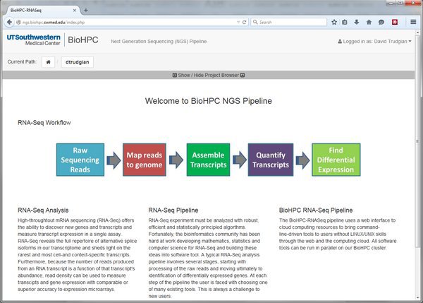
Home Page
The NGS pipeline homepage gives some basic information about the system. There are three important areas in the menu bar of the system, indicated by the red labels below:
User Menu: This menu allows you to logout from the system, and contains a user profile link that will be used to manage user settings in future.
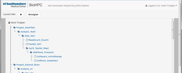
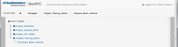
Current Project Path: As we'll see later, data is analyzed in projects, and each project contains a tree of modules which are run to perform certain tasks. The output of one module might become the input of another. Some modules are dead-ends. Your current location in the structure of a project is displayed in the current path bar, and you can click the links to navigate back up in the project structure.
Project Browser: The project browser (usually hidden) shows the complete tree-structure of your projects, letting you navigate to any part of any project quickly. To use it click on the 'show/hide' link:
Projects, Analyses, Data, and Modules
Before we start work, let's examine how the NGS system structures a project:
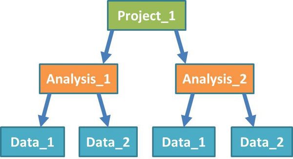
Projects: A project sits at the top level in the system. You can group any work that is related to an experimental project together, inside an NGS pipeline project.
Analysis: Each project will contain one or more analyses. Analyses may involve multiple datasets, but work on these datasets is usually related in some way.
Data: Within each analysis are one or more datasets, on which the pipeline tools will be run. Datasets can include input files from different experimental groups. You shouldn't separate out groups that you want to compare directly into different datasets.
Modules: (Not shown in diagram) Modules are components of the analysis pipeline which run software tools on input data, or the output of preceding modules. They perform functions such as mapping short reads from an RNA-Seq experiment to a reference genome, or looking for significant expression differences between quantified transcripts from different groups of samples.
Our Test Dataset
Let's create a simple test project. We're going to work to compare the expression of genes/transcripts between adrenal gland and brain samples. We have RNASeq data as raw .fastq sequence files, and we want to ultimately obtain a list of genes/transcripts that have significantly different expression between our samples. FastQ files are the standard for raw read data obtained from a sequencing platform. Your input to the pipeline must be in fastq format, and can optionally be compressed to save space using gzip as a .fastq.gz file.
Our test dataset will be very small, so we don't use a waste a lot of compute time, and we can work through the entire pipeline quickly. We will borrow the data from the Galaxy project. Download the 4 .fastq files from the Galaxy RNASeq tutorial page:
https://usegalaxy.org/u/jeremy/p/galaxy-rna-seq-analysis-exercise
Copy, or save these files into your project directory on BioHPC.
The 4 files form 2 pairs, as the RNASeq data was acquired in a paired-end experiment, where fragmented sequences are read at both ends by the sequencer. adrenal_1.fastq and adrenal_2.fastq contain the forward and reverse short-reads from our adrenal sample. We also have paired files for our brain sample.
These files are small extracts from a large sequencing experiment, containing reads around a specific region of Chr19 that were extracted from a complete RNASeq dataset for tutorial purposes. Each file is around 8Mbytes. Typically the fastq files you will receive from an RNASeq experiment are multiple gigabytes in size.
For the rest of this tutorial we're assuming the datasets have been copied into /project/biohpcadmin/dtrudgian/rna_seq_de which is in my project area on BioHPC storage system. Where file paths are used you must adjust them to reflect where you downloaded or copied the files.
IMPORTANT: This is an example analysis, where we have only a single sequencing dataset per group. We can work through the pipeline without replicates, but you should generally obtain relevant replicate datasets in real experiments. Differential expression tools will be more accurate and sensitive when they are able to observe variation between replicate samples, and use this information to decide what a significant difference really is.
Create a New Project
We'll create a new project now. Scroll to the bottom of the homepage and click the Go to NGS Pipeline button. A table will be displayed that will list all of our RNASeq experiments (if we have any). Choose Create a New Project and fill in the basic details:
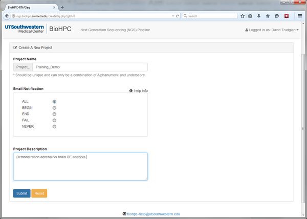
The Project Name and Project Description are self-explanatory. The Email Notification option is more cryptic. Throughout the pipeline you will notice help icons and links. If you click one of these it will give you an explanation of the relevant options:
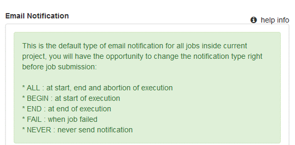
Our pipeline modules will submit jobs to the BioHPC nucleus cluster. The Email Notification option lets us ask the cluster to inform us when a job begins, ends, fails, all of these, or not at all. When running analyses with large datasets email notifications can be useful to let us know when something has finished and we can proceed to the next step of the pipeline.
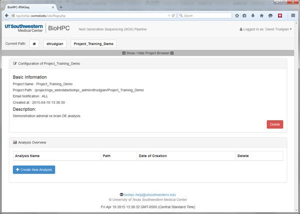
Submit the form and our new project will be displayed. Look at the current project path bar and the project browser. Notice that we are now within this project, and it has appeared in the project tree.
Start an Analysis within Our Project
Our project might be large, complex, consisting of many different experiments. We can create many Analyses within our project to organize these. Go ahead and create a new analysis with a sensible name:
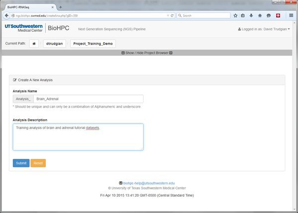
When you've submitted the form you'll notice from the project path that we're now inside the analysis. In the tree we have an extra level. Project->Analysis.
Remember that you can move around inside your projects using the links in the current path, or the project browser tree.
Creating these project and analysis levels might seem tedious, but we are only working on a small test analysis. When you have a big project the different levels in the tree allow you to keep your data and results clearly organized within the NGS pipeline system.
Adding Data
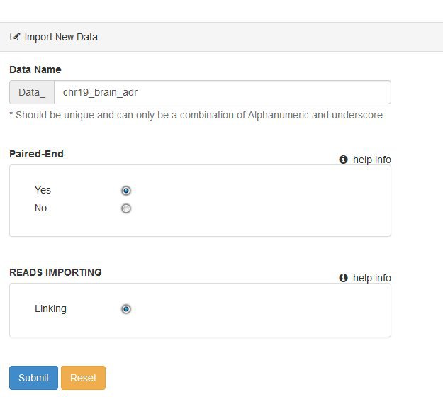
We now need to add new data for our analysis. Click the Create New Data button and fill in the basic information about the dataset you want to use.
For the tutorial our data is paired-end, so answer yes to that question.
Ignore the Reads Importing option for now - this relates to plans to include other ways of getting data into the pipeline.
Once you submit the form you'll see the same table of basic information that we saw for the project and analysis levels. We now have an additional set of tabs above the basic information, but we'll get back to these shortly. First we need to tell the system where our data files are on the BioHPC storage. This is done using a manifest file. The manifest is simply a list of input .fastq files, and the experimental source / groups / replicate structure they each belong to.
There are two ways to create a manifest:
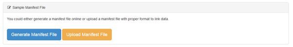
We can either Generate our manifest file, in which case we'll be creating it using an online form, or Upload one. Unless you have a lot of data files you will want to Generate the file using the form, which is easier. If you have a lot of files, groups, replicates in a complicate experimental structure it may be easier to assemble the manifest file in e.g. Excel, then upload it. If you choose the Upload option there's a help screen that explains how to do that.
Let's create our manifest online. Go ahead and click the Generate Manifest File button.
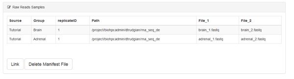
You'll see a blank form, where you have the option to Add Samples. We have two samples (each with paired input files) so go ahead and click the Add Sample button twice. Here's the manifest completed - we'll explain it below:
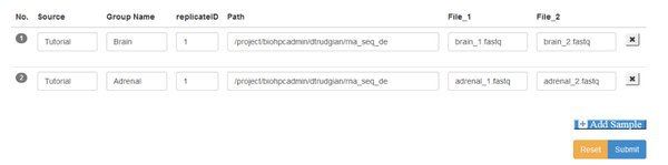
Source This box is to record the origin of the sample, however makes sense for your study.
Group You must assign samples to groups. The groups categorize your samples so that you can compare between groups. Here we have a brain group and an adrenal group, each with only replicate sample. Your can have any number of groups, containing one or more replicate samples.
replicateID Each replicate within a group must have a unique ID. You can use the same replicate IDs in different groups.
Path This is the path or directory where your data files are stored on the cluster. You must provide the full path, excluding the filename. Your samples might each come from a different path, or all be in the same directory. If using paired end data the paired files for a sample must be in the same directory.
File 1/2 If your data is single-end there will be a single File1 box, to enter the filename for the .fastq file that holds the short-read sequences for that sample. If you are working with paired-end data there will be File1 and File2 boxes, to enter the forward and reverse read filenames respectively.
When you have completed the manifest form click Submit. You'll go back to the data summary page, which will now list the samples you entered into the manifest. They aren't yet linked to the system. Go ahead and click the Link button. You also have an option to delete the manifest file if you need to start over.
On clicking Link the system checks for the existence of all the files specified. If no error is displayed you can proceed. Otherwise you'll need to correct your manifest.
The File Folder and Next Tabs
Above our data information table we saw some additional tabs, named File Folder and Next. These will appear on any 'Data' section, or when we are working with modules that process data.
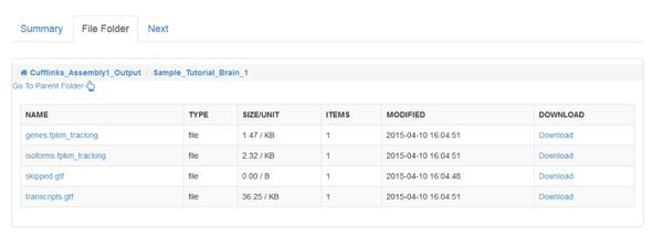
File Folder
Click on the File Folder tab and have a look around. You'll see files and folders that you can browse in and out of. They'll contain input data, output data, log messages and scripts. You don't need to worry about most of these. We'll come back to this tab when we open up some output from a module later on.
Next
The Next tab list the things we can do, given that we are currently looking at a dataset. Each of the options listed is a different module that does a certain job. We can choose a module to run it against the dataset we are currently working on.
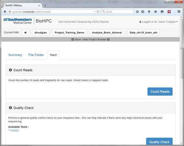
Here we can see options to Count Reads or Quality Check our data. There are more options below. Whenever you go to the 'Next' tab it will show the modules that are valid to run, depending on where you are in the pipeline. At the moment we see all the modules that can be run against our raw input data. Later we will map our reads to the genome. After that the 'Next' tab will list modules that can be run against mapped reads. If you don't see the options you expect, check that you are in the right location in the pipeline by looking at the Current Path bar. You can use the Project Browser to move around if you need to go somewhere else.
Count Reads
The Count Reads module does exactly that - just counts the number of short-read sequences we have in our input files. Most of the time we'll be given a report by a sequencing facility with our data, so we don't need to count the reads at the start of our pipeline. The option is there though, if you wish. Counting reads might be more useful when you have trimmed or processed data, and you need to see how many reads remain. We'll skip counting reads for now.
Quality Check
Sequencing facilities will often give their customers a QC report, or some information about the quality of their data. However, it's always a good idea to QC check your input data to a pipeline, just to check for anything that might explain problems later on.
Go ahead and click the Quality Check button. We're going to run the Quality Check module on our data. This module uses the program FastQC to produce a report on each input data file.
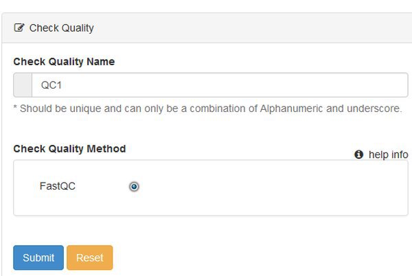
When we choose a module we see a form that lets us name the run, and choose any options. There's nothing to choose for QC, so just submit the form.
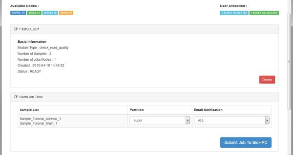
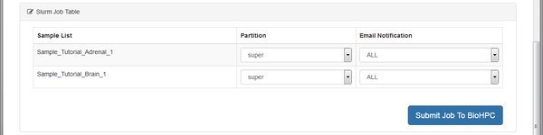
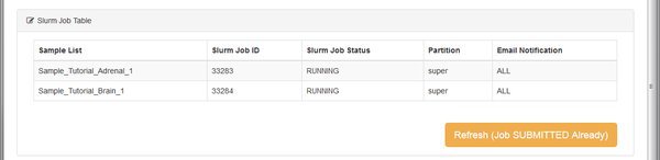
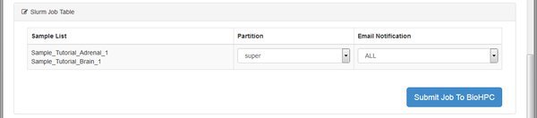
The QC module is going to run on the BioHPC cluster. We see the basic details for the module, and then a table listing the cluster (SLURM) jobs that the system will submit. For each job we can choose a specific cluster partition, and email notification setting. You can leave these alone - the RNASeq modules don't require any special settings here. Just click Submit Job To BioHPC so that our QC run is sent to the cluster for processing.
Depending on the cluster queue and the complexity of the job, it can take a while for a module to finish running. If you have email notifications enabled you can get on with something else, wait for the email, then come back to the NGS pipeline to look at results or move to the next step of your analysis.
Our example data files are very small, so if the cluster has free nodes the job finishes quickly. We can press the Refresh button on the page to check the status of the job. Once all jobs listed for a module are COMPLETED then we can look at output, take next steps in the pipeline etc.
Wait until your job is done, refresh, and then we can look at the output of this QC module.
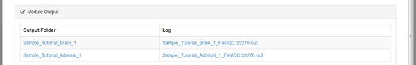
Some modules run the same tool on each sample or input file. Some modules will merge data together. The number of outputs listed depends on what the module is doing. To look at outputs, click on one of the Output Folder links.
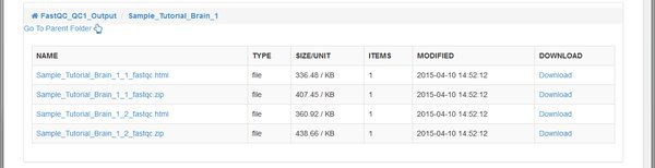
The QC tool has created an HTML report, and a .zip file for each of our paired input .fastq files belonging to the Tutorial_Brain_1 sample. The .zip file is an archive of the report that you can download and extract if you want to open it on your computer.
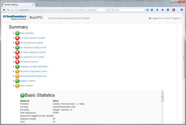
Open the .html report by clicking on the link and we'll see the QC report for this input file of short-reads. In this example there are a lot of red crosses. Many of these are because this data is just a very small extract from a larger dataset. On such a small and selective extract we don't expect nice even distribution of bases etc. You should speak to your sequencing core about interpreting the report for your input data.
We've now gone through the process of running a module within the pipeline. It's always the same basic process. Select a module from the Next tab, choose parameters, submit to the cluster, wait and view output.
Mapping Reads to the Genome
In our pipeline to find differentially expressed genes/transcripts we need to:
-
(Optional) filter/trim our input data
-
Map our reads for each sample to the genome
-
(Optional) Filter our mapped reads, to remove low quality mappings.
-
Assemble our mapped reads into a list of transcripts for each sample
-
Merge the lists of transcripts into a master list
-
Quantify the abundance of transcripts in each group
-
Find the significantly differentially expressed genes and transcripts.
Let's start at the beginning. If using a real dataset we might want to filter our input data, using the Reads Trimming module. This removes low quality reads from consideration. It can take a long time to map low quality reads to the genome, and the mappings are usually inaccurate. By filtering them out before mapping we save time, and reduce the number of incorrect mappings. In this example we will not filter our reads because of our small test dataset.
We'll go ahead and map our short reads to the genome to see which parts of the genome our RNASeq experiment observed as being transcribed. You might still be looking at the QC module we ran earlier. The QC output is a dead-end. We need to go back to our Data and run the read mapping module from there - it uses our original .fastq files as input.
Use the Project Browser or Current Path buttons to navigate back to our Data. Then go to the Next tab, to access the list of modules we could run. We are now going to choose to Map Reads.
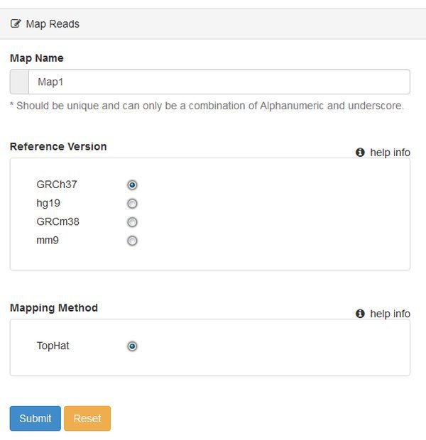
You'll be asked to select a Reference Version - which is the genome / annotation that you want to use. This is human data, so let's choose hg19, which will use the UCSC hg19 sequence and annotation files. At present you can only map reads using TopHat. The pipeline will use TopHat version 2.x with default options.
Mapping can take a long time on large files, so the module will create a cluster job for each sample. If there's space in the cluster queue the mapping processes can run in parallel, using more than one node. Submit the jobs, wait and refresh until the work is done.
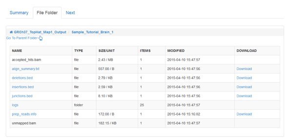
When the jobs are all COMPLETED we can inspect the output, as we did for the QC module. However, the main output of read mapping isn't very interesting to us - it's a large .bam file, which has a binary format encoding of the alignments that were found. The most interesting file for us to look at is the align_summary.txt which gives statistics about the number of reads that could be aligned, etc:
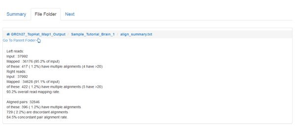
The percentage of mapped reads that can be considered 'good' depends on your sample and the sequencing technique. Speak to your sequencing provider if you have doubts.
If you go to the Next tab for our completed mapping module you'll see that there are a number of things we can do with our mapped reads. We can Count Reads which will tell us how many were mapped/unmapped etc. We can Process Mapped Reads to filter out low quailty mappings before assembling them into transcripts, or we can directly Assemble Reads into transcripts.
Processing Mapped Reads
We'll go ahead and Process Mapped Reads to remove low quality mappings before we assemble them into transcripts. If our mapping output contains low quality incorrect read to genome mappings it will slow down transcript assembly, and potentially lead to less useful results. Following the general procedure before, run the Process Mapped Reads module on our dataset. There are no options to set. When the job has run, continue to the next step….
Assemble Reads
We now have our short reads aligned to the genome, and we have filtered out any low quality mappings. Because we want to quantify transcripts or genes, and not just count reads vs genome location, we must assemble our reads into transcripts. The NGS pipeline uses the Cufflinks tool suite to assemble reads into transcripts, quantify them, and perform differential expression. Let's begin this process by running the Assemble Reads module against our filtered mapped reads. The cufflinks tool will examine the structure of our mapped reads, the overlaps between reads, covered vs non-covered regions of the genome, to assemble a list of transcripts.
Follow the standard procedure to create and submit the Assemble Reads module from the Next tab.
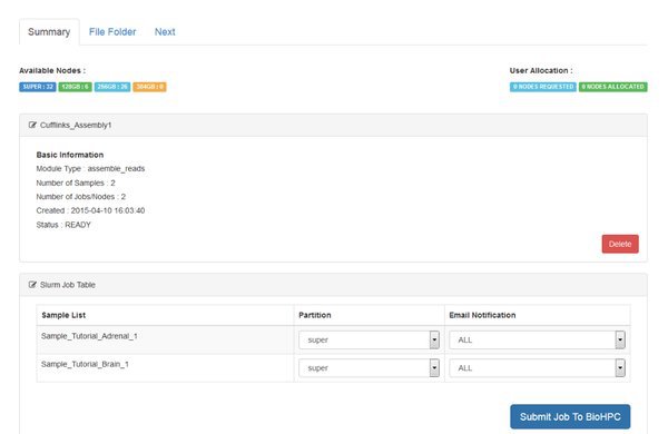
Notice that two jobs are being submitted to the cluster. Cufflinks is run separately for each sample in our data. For every sample it will generate an output file called 'transcripts.gtf'. This is an annotation file which lists the genomic locations for the transcripts that cufflinks was able to assemble from our mapped reads.
We need to merge these annotation files before we quantify across all of our samples. You'll find a module called Cuffmerge Transcripts in the Next tab to do this.
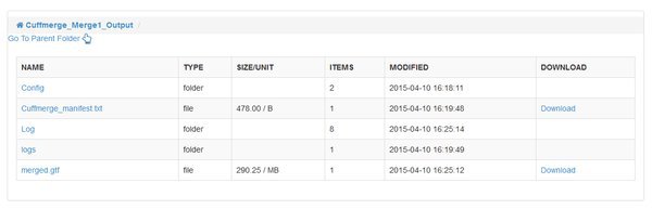
CuffMerge Transcripts
The CuffMerge Transcipts module has no additional options, and should run fairly quickly. When it is complete notice that it has a single output folder. Up until this point we had outputs for each input sample, but cuffmerge has joined the list of transcripts for each sample into a single, consistent 'merged.gtf' output file. Any differences in transcript assembly for our individual samples are reconciled, so we have a high quality final assembly that is consistent across the entirety of our data. The module will also bring in information from a reference annotation of the genome, so that the .gtf file includes familiar gene names etc.
Quantify Mapped Reads / Cuffquant
Once the merged transcript assembly is computed we can quantify our transcripts for each sample, with respect to the merged assembly. This step is performed by a module called Quantify Mapped Reads which uses the cuffquant tool from the Cufflinks suite. Cuffquant takes as input the file merged.gtf transcript assembly, and our original mapped reads output from the TopHat aligner. The output is transcript-level quantitation for each of our samples, ready to perform differential expression analysis. The module runs one job per sample, so that the transcript quantitation can be run in parallel on the BioHPC cluster:
The output from cuffquant is a .cxb file for each sample. These .cxb files are a special cufflinks format, containing transcript abundances. When the module is complete we have two options on the Next tab:
Normalize Quantified Reads: this module will normalize the quantified reads across your samples, to give output in a format that can be download and used for downstream analysis. The output is a series of tables that can be loaded into Excel, R, and other tools.
Differential Expression: the differential expression module performs a statistical analysis of the abundances of transcripts and genes in each sample, to identify significant differences between groups. The final output is a list of significantly differently expressed genes and transcripts.
Differential Expression
In this example we will use the Differential Expression module to obtain our list of DE genes and transcripts. The module uses the cuffdiff program from the cufflinks suite of tools. Choose the Differential Expression modules from the Next tab, and you will be presented with a parameter screen:
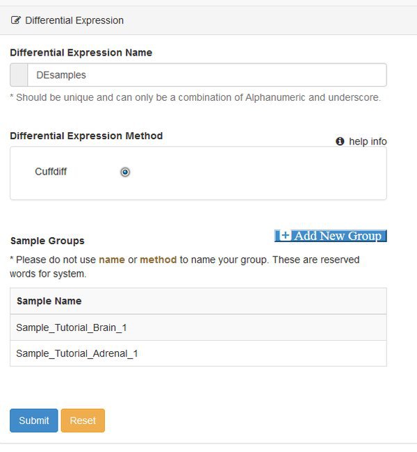
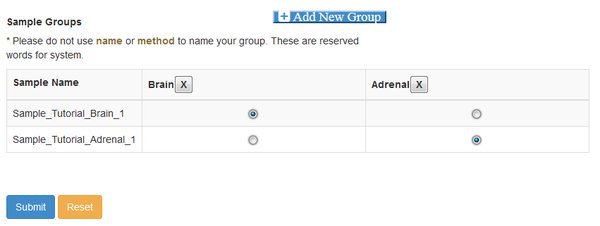
At this point you need to define groups of samples, to control the comparisons that cuffdiff will make. Cuffdiff will look for significant differential expression between all possible pairs of groups that you define. Here we only have two groups, so we click Add New Group twice and fill out the resulting form. Enter the names you want to use for each group, confirm the names by clicking the check box, and then assign each sample to a group with the matrix of radio buttons:
Note that if you have a complex experiment with many conditions, and you want to make different sets of comparisons of differential expression, you could run the Differential Expression module multiple time. A different grouping can be set each time the module is run.
Once the groups are selected properly submit the parameter form, and then submit the job to the cluster on the next page.
This step of the pipeline generally runs quickly, if the cluster has available nodes. The output from this module is the final output from our differential expression pipeline. Cuffdiff generates a number of output tables, each containing useful results.
A full explanation of the different output files is given in the cuffdiff manual online (http://cole-trapnell-lab.github.io/cufflinks/cuffdiff/#cuffdiff-output-files). Generally the following outputs are most interesting in standard differential expression experiments:
genes.fpkm_tracking / isoforms.fpkm_tracking: These files contain tables of quantitative FPKM information, representing the relative abundance of each gene/transcript in each sample.
genes.count_tracking / isoforms.count_tracking: The same as the FPKM files above, but using fragment counts instead of FPKM as the quantitative measure.
isoform_exp.diff / gene_exp.diff: Differential expression results - contain the results of tests for significant difference in expression for each gene/transcript, between each of the defined groups.
Download the gene_exp.diff file, and open it in Excel. When you double click the file you might need to specifically choose Excel to open it - or you can drag it onto an Excel window.
Within Excel sort the table of values by the 'q-value' column, from smallest to largest. The q-value is computed from the p-value to correct for multiple testing. A small q-value means that DE is more likely to be true for the relevant gene.
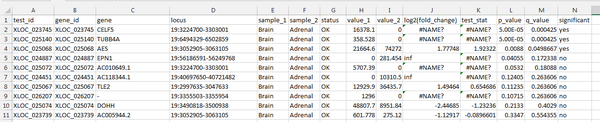
In our output, there are 3 genes with significant DE between adrenal and brain samples, according to the cufflinks analysis. Remember that this data is a small extract - so not many genes were seen total.
CELF5 shows significant DE. The quantitative FPKM value is high for brain, and 0 in adrenal tissue. This is an expected finding - CELF5 is selectively expressed in the cerebral cortex.