R on BioHPC - A quick look at Bioconductor
We’re going to take a brief tour of some of the most useful aspects of Bioconductor for common RNASeq and ChipSEQ data analysis tasks.
If you are using the BioHPC RStudio server, or the R/3.2.1-intel module you should have all required packages available. If using your own computer you will need to install the neccessary packages from Bioconductor by running the commented code below:
# Install packages - uncomment and run this code if R cannot find a package.
# source("http://bioconductor.org/biocLite.R")
# biocLite(c('airway','Rsamtools','GenomicFeatures','GenomicAlignments','DESeq2','rtracklayer','pheatmap','BSgenome.Hsapiens.UCSC.hg19','org.Hs.eg.db','AnnotationDbi'))
RNA-Seq Differential Expression with DESeq
The airway package contains a small subset of the RNA-Seq data from a study of airway muscle cells treated with a synthetic steroid. The data was originally obtained from:
Himes BE, Jiang X, Wagner P, Hu R, Wang Q, Klanderman B, Whitaker RM, Duan Q, Lasky-Su J, Nikolos C, Jester W, Johnson M, Panettieri R Jr, Tantisira KG, Weiss ST, Lu Q. “RNA-Seq Transcriptome Profiling Identifies CRISPLD2 as a Glucocorticoid Responsive Gene that Modulates Cytokine Function in Airway Smooth Muscle Cells.” PLoS One. 2014 Jun 13;9(6):e99625. PMID: 24926665. GEO: GSE52778.
The analysis presented here is a shortened and (slightly) modified version of the bioconductor rnaseqGene workflow, which can be found online at:
http://www.bioconductor.org/help/workflows/rnaseqGene/
The original workflow is distributed under the Artistic License and was authored by:
Michael Love [1], Simon Anders [2], Wolfgang Huber [2]
- [1] Department of Biostatistics, Dana-Farber Cancer Institute and Harvard School of Public Health, Boston, US;
- [2] European Molecular Biology Laboratory (EMBL), Heidelberg, Germany.
We stronly suggest taking a look at the original workflow, and the others available on the Bioconductor site. They cover a significant number of common tasks you are likely carry out.
http://www.bioconductor.org/help/workflows/
Loading data
As we mentioned, the Bioconductor package airway contains the sample data for this workflow. The package consists of aligned reads for a portion of the data from a small region of the genome. This will let us look at preparing this type of data for downstream analysis quickly and easily. The package also contains a pre-prepared object created from the entire experiment that we’ll pick up for later portions of the exercise.
First, we load the library then find and list the contents of it’s extdata directory.
library("airway")## Loading required package: GenomicRanges
## Loading required package: BiocGenerics
## Loading required package: parallel
##
## Attaching package: 'BiocGenerics'
##
## The following objects are masked from 'package:parallel':
##
## clusterApply, clusterApplyLB, clusterCall, clusterEvalQ,
## clusterExport, clusterMap, parApply, parCapply, parLapply,
## parLapplyLB, parRapply, parSapply, parSapplyLB
##
## The following object is masked from 'package:stats':
##
## xtabs
##
## The following objects are masked from 'package:base':
##
## anyDuplicated, append, as.data.frame, as.vector, cbind,
## colnames, do.call, duplicated, eval, evalq, Filter, Find, get,
## intersect, is.unsorted, lapply, Map, mapply, match, mget,
## order, paste, pmax, pmax.int, pmin, pmin.int, Position, rank,
## rbind, Reduce, rep.int, rownames, sapply, setdiff, sort,
## table, tapply, union, unique, unlist, unsplit
##
## Loading required package: S4Vectors
## Loading required package: stats4
## Loading required package: IRanges
## Loading required package: GenomeInfoDbdir <- system.file("extdata", package="airway", mustWork=TRUE)
list.files(dir)## [1] "GSE52778_series_matrix.txt"
## [2] "Homo_sapiens.GRCh37.75_subset.gtf"
## [3] "sample_table.csv"
## [4] "SraRunInfo_SRP033351.csv"
## [5] "SRR1039508_subset.bam"
## [6] "SRR1039509_subset.bam"
## [7] "SRR1039512_subset.bam"
## [8] "SRR1039513_subset.bam"
## [9] "SRR1039516_subset.bam"
## [10] "SRR1039517_subset.bam"
## [11] "SRR1039520_subset.bam"
## [12] "SRR1039521_subset.bam"There are a number of .bam files containing aligned RNA-Seq reads, .csv files containing the experimental design, and a .gtf file containing a subset of gene co-ordinates corresponding to the reduced set of aligned reads.
We can go ahead and load the sample information, and then obtain a list of the bam files we’d like to work with.
csvfile <- file.path(dir,"sample_table.csv")
(sampleTable <- read.csv(csvfile,row.names=1))
## SampleName cell dex albut Run avgLength Experiment
## SRR1039508 GSM1275862 N61311 untrt untrt SRR1039508 126 SRX384345
## SRR1039509 GSM1275863 N61311 trt untrt SRR1039509 126 SRX384346
## SRR1039512 GSM1275866 N052611 untrt untrt SRR1039512 126 SRX384349
## SRR1039513 GSM1275867 N052611 trt untrt SRR1039513 87 SRX384350
## SRR1039516 GSM1275870 N080611 untrt untrt SRR1039516 120 SRX384353
## SRR1039517 GSM1275871 N080611 trt untrt SRR1039517 126 SRX384354
## SRR1039520 GSM1275874 N061011 untrt untrt SRR1039520 101 SRX384357
## SRR1039521 GSM1275875 N061011 trt untrt SRR1039521 98 SRX384358
## Sample BioSample
## SRR1039508 SRS508568 SAMN02422669
## SRR1039509 SRS508567 SAMN02422675
## SRR1039512 SRS508571 SAMN02422678
## SRR1039513 SRS508572 SAMN02422670
## SRR1039516 SRS508575 SAMN02422682
## SRR1039517 SRS508576 SAMN02422673
## SRR1039520 SRS508579 SAMN02422683
## SRR1039521 SRS508580 SAMN02422677filenames <- file.path(dir, paste0(sampleTable$Run, "_subset.bam"))The Rsamtools package provides facilities for reading bam and sam files into R, and working with them. In this case we can read our list of bam files in a single step. The yieldSize parameter specifies that the files should be processed 2,000,000 reads at a time. With very large datasets this is important to avoid overwhelming the memory on smaller machines.
library("Rsamtools")## Loading required package: XVector
## Loading required package: Biostringsbamfiles <- BamFileList(filenames, yieldSize=2000000)Now that the reads are loaded we can check the chromosome names that were used in the alignment. We’ll see either chr_1 or 1 depending on which naming scheme was used. The names used in the alignment must match those in the gene information we will match to our reads.
seqinfo(bamfiles[1])## Seqinfo object with 84 sequences from an unspecified genome:
## seqnames seqlengths isCircular genome
## 1 249250621 <NA> <NA>
## 10 135534747 <NA> <NA>
## 11 135006516 <NA> <NA>
## 12 133851895 <NA> <NA>
## 13 115169878 <NA> <NA>
## ... ... ... ...
## GL000210.1 27682 <NA> <NA>
## GL000231.1 27386 <NA> <NA>
## GL000229.1 19913 <NA> <NA>
## GL000226.1 15008 <NA> <NA>
## GL000207.1 4262 <NA> <NA>Assigning and Counting Read per Gene
Our reads from the bam files are assigned co-ordinates on the chromosomal sequences. In order to look at gene expression we must assign the reads to genes, and count the number assigned to each gene.
The GenomicFeatures library contains functions that allow us to create databases of features from various types of inputs. Here we will create a database of transcripts within R, loading gene information from a GTF file. With this database we can then create a list of all exons, grouped by gene, which we’ll use to assign our reads to genes.
library("GenomicFeatures")## Loading required package: AnnotationDbi
## Loading required package: Biobase
## Welcome to Bioconductor
##
## Vignettes contain introductory material; view with
## 'browseVignettes()'. To cite Bioconductor, see
## 'citation("Biobase")', and for packages 'citation("pkgname")'.gtffile <- file.path(dir,"Homo_sapiens.GRCh37.75_subset.gtf")
(txdb <- makeTxDbFromGFF(gtffile, format="gtf"))## Warning in matchCircularity(seqlevels(gr), circ_seqs): None of the strings
## in your circ_seqs argument match your seqnames.## Prepare the 'metadata' data frame ... metadata: OK## TxDb object:
## # Db type: TxDb
## # Supporting package: GenomicFeatures
## # Data source: C:/Users/dtrudg/Documents/R/win-library/3.2/airway/extdata/Homo_sapiens.GRCh37.75_subset.gtf
## # Organism: NA
## # miRBase build ID: NA
## # Genome: NA
## # transcript_nrow: 65
## # exon_nrow: 279
## # cds_nrow: 158
## # Db created by: GenomicFeatures package from Bioconductor
## # Creation time: 2015-07-14 14:25:50 -0500 (Tue, 14 Jul 2015)
## # GenomicFeatures version at creation time: 1.20.1
## # RSQLite version at creation time: 1.0.0
## # DBSCHEMAVERSION: 1.1(exonsByGene <- exonsBy(txdb, by="gene"))## GRangesList object of length 20:
## $ENSG00000009724
## GRanges object with 18 ranges and 2 metadata columns:
## seqnames ranges strand | exon_id exon_name
## <Rle> <IRanges> <Rle> | <integer> <character>
## [1] 1 [11086580, 11087705] - | 98 ENSE00000818830
## [2] 1 [11090233, 11090307] - | 99 ENSE00000472123
## [3] 1 [11090805, 11090939] - | 100 ENSE00000743084
## [4] 1 [11094885, 11094963] - | 101 ENSE00000743085
## [5] 1 [11097750, 11097868] - | 103 ENSE00003520086
## ... ... ... ... ... ... ...
## [14] 1 [11106948, 11107176] - | 111 ENSE00003467404
## [15] 1 [11106948, 11107176] - | 112 ENSE00003489217
## [16] 1 [11107260, 11107280] - | 113 ENSE00001833377
## [17] 1 [11107260, 11107284] - | 114 ENSE00001472289
## [18] 1 [11107260, 11107290] - | 115 ENSE00001881401
##
## ...
## <19 more elements>
## -------
## seqinfo: 1 sequence from an unspecified genome; no seqlengthsWe generate our counts by looking at how many reads overlap the co-ordinates of exons which we know belong to a specific gene. TheGenomicAlignments package contains a summarizeOverlaps function to do this:
library("GenomicAlignments")
library("BiocParallel")
register(SerialParam())

se <- summarizeOverlaps(features=exonsByGene, reads=bamfiles,
                        mode="Union",
                        singleEnd=FALSE,
                        ignore.strand=TRUE,
                        fragments=TRUE )
Our output se is a summarized experiment object. Let’s look at some of the gene counts, and the summed counts of reads assigned to any gene in each sample.
head(assay(se))## SRR1039508_subset.bam SRR1039509_subset.bam
## ENSG00000009724 38 28
## ENSG00000116649 1004 1255
## ENSG00000120942 218 256
## ENSG00000120948 2751 2080
## ENSG00000171819 4 50
## ENSG00000171824 869 1075
## SRR1039512_subset.bam SRR1039513_subset.bam
## ENSG00000009724 66 24
## ENSG00000116649 1122 1313
## ENSG00000120942 233 252
## ENSG00000120948 3353 1614
## ENSG00000171819 19 543
## ENSG00000171824 1115 1051
## SRR1039516_subset.bam SRR1039517_subset.bam
## ENSG00000009724 42 41
## ENSG00000116649 1100 1879
## ENSG00000120942 269 465
## ENSG00000120948 3519 3716
## ENSG00000171819 1 10
## ENSG00000171824 944 1405
## SRR1039520_subset.bam SRR1039521_subset.bam
## ENSG00000009724 47 36
## ENSG00000116649 745 1536
## ENSG00000120942 207 400
## ENSG00000120948 2220 1990
## ENSG00000171819 14 1067
## ENSG00000171824 748 1590colSums(assay(se))## SRR1039508_subset.bam SRR1039509_subset.bam SRR1039512_subset.bam
## 6478 6501 7699
## SRR1039513_subset.bam SRR1039516_subset.bam SRR1039517_subset.bam
## 6801 8009 10849
## SRR1039520_subset.bam SRR1039521_subset.bam
## 5254 9168We need to remember to add the sample table into the summarized experiment, placing it into colData. Without doing this the se object doesn’t contain any information about our experimental conditions, only sample identifiers.
(colData(se) <- DataFrame(sampleTable))## DataFrame with 8 rows and 9 columns
## SampleName cell dex albut Run avgLength
## <factor> <factor> <factor> <factor> <factor> <integer>
## SRR1039508 GSM1275862 N61311 untrt untrt SRR1039508 126
## SRR1039509 GSM1275863 N61311 trt untrt SRR1039509 126
## SRR1039512 GSM1275866 N052611 untrt untrt SRR1039512 126
## SRR1039513 GSM1275867 N052611 trt untrt SRR1039513 87
## SRR1039516 GSM1275870 N080611 untrt untrt SRR1039516 120
## SRR1039517 GSM1275871 N080611 trt untrt SRR1039517 126
## SRR1039520 GSM1275874 N061011 untrt untrt SRR1039520 101
## SRR1039521 GSM1275875 N061011 trt untrt SRR1039521 98
## Experiment Sample BioSample
## <factor> <factor> <factor>
## SRR1039508 SRX384345 SRS508568 SAMN02422669
## SRR1039509 SRX384346 SRS508567 SAMN02422675
## SRR1039512 SRX384349 SRS508571 SAMN02422678
## SRR1039513 SRX384350 SRS508572 SAMN02422670
## SRR1039516 SRX384353 SRS508575 SAMN02422682
## SRR1039517 SRX384354 SRS508576 SAMN02422673
## SRR1039520 SRX384357 SRS508579 SAMN02422683
## SRR1039521 SRX384358 SRS508580 SAMN02422677We now have a complete set of read counts across each of our samples. We started with a subset of data from the real experiment for speed, so let’s load a pre-computed dataset that covers the entirity of the experimental data. We’ll check how many million reads aligned to genes in each of the samples.
data("airway")
se <- airway

round( colSums(assay(se)) / 1e6, 1 )
## SRR1039508 SRR1039509 SRR1039512 SRR1039513 SRR1039516 SRR1039517
## 20.6 18.8 25.3 15.2 24.4 30.8
## SRR1039520 SRR1039521
## 19.1 21.2The experimental setup is alrady present in the colData slot. We have cell line and treatment information for each sample, and can continue to differential expression analysis.
colData(se)## DataFrame with 8 rows and 9 columns
## SampleName cell dex albut Run avgLength
## <factor> <factor> <factor> <factor> <factor> <integer>
## SRR1039508 GSM1275862 N61311 untrt untrt SRR1039508 126
## SRR1039509 GSM1275863 N61311 trt untrt SRR1039509 126
## SRR1039512 GSM1275866 N052611 untrt untrt SRR1039512 126
## SRR1039513 GSM1275867 N052611 trt untrt SRR1039513 87
## SRR1039516 GSM1275870 N080611 untrt untrt SRR1039516 120
## SRR1039517 GSM1275871 N080611 trt untrt SRR1039517 126
## SRR1039520 GSM1275874 N061011 untrt untrt SRR1039520 101
## SRR1039521 GSM1275875 N061011 trt untrt SRR1039521 98
## Experiment Sample BioSample
## <factor> <factor> <factor>
## SRR1039508 SRX384345 SRS508568 SAMN02422669
## SRR1039509 SRX384346 SRS508567 SAMN02422675
## SRR1039512 SRX384349 SRS508571 SAMN02422678
## SRR1039513 SRX384350 SRS508572 SAMN02422670
## SRR1039516 SRX384353 SRS508575 SAMN02422682
## SRR1039517 SRX384354 SRS508576 SAMN02422673
## SRR1039520 SRX384357 SRS508579 SAMN02422683
## SRR1039521 SRX384358 SRS508580 SAMN02422677Differential Expression Analysis with DESeq2
We will use the DESeq2 package to identify genes that are expressed differently between cell lines and treatments. We start by loading the library, and then setting up a DESeqDataSet object with our count information from se. We tell DESeq that our experimental design uses two factors, cell line and dex treatment so we’re interested in considering differences between the relevant subsets of samples.
library("DESeq2")## Loading required package: Rcpp
## Loading required package: RcppArmadillodds <- DESeqDataSet(se, design = ~ cell + dex)Before running the DESeq2 analysis we’ll look at the data interactively with some plots. First we apply a regularized log transform. This is a transformation that shrinks low value counts for a gene toward the mean across all samples. This addresses the issue of heteroskedastic data, where the variance of the counts depends on their magnitude. It’s a useful transformation for exploring the data, but the DESeq2 run itself will run on the raw counts.
rld <- rlog(dds)
head(assay(rld))
## SRR1039508 SRR1039509 SRR1039512 SRR1039513 SRR1039516
## ENSG00000000003 9.399151 9.142478 9.501695 9.320796 9.757212
## ENSG00000000005 0.000000 0.000000 0.000000 0.000000 0.000000
## ENSG00000000419 8.901283 9.113976 9.032567 9.063925 8.981930
## ENSG00000000457 7.949897 7.882371 7.834273 7.916459 7.773819
## ENSG00000000460 5.849521 5.882363 5.486937 5.770334 5.940407
## ENSG00000000938 -1.638084 -1.637483 -1.558248 -1.636072 -1.597606
## SRR1039517 SRR1039520 SRR1039521
## ENSG00000000003 9.512183 9.617378 9.315309
## ENSG00000000005 0.000000 0.000000 0.000000
## ENSG00000000419 9.108531 8.894830 9.052303
## ENSG00000000457 7.886645 7.946411 7.908338
## ENSG00000000460 5.663847 6.107733 5.907824
## ENSG00000000938 -1.639362 -1.637608 -1.637724Let’s go ahead and compute the euclidean distance between samples and plot it in a heatmap to visualize their overall similarity.
sampleDists <- dist( t( assay(rld) ) )
sampleDists
## SRR1039508 SRR1039509 SRR1039512 SRR1039513 SRR1039516
## SRR1039509 40.89060
## SRR1039512 37.35231 50.07638
## SRR1039513 55.74569 41.49280 43.61052
## SRR1039516 41.98797 53.58929 40.99513 57.10447
## SRR1039517 57.69438 47.59326 53.52310 46.13742 42.10583
## SRR1039520 37.06633 51.80994 34.86653 52.54968 43.21786
## SRR1039521 56.04254 41.46514 51.90045 34.82975 58.40428
## SRR1039517 SRR1039520
## SRR1039509
## SRR1039512
## SRR1039513
## SRR1039516
## SRR1039517
## SRR1039520 57.13688
## SRR1039521 47.90244 44.78171library("pheatmap")
library("RColorBrewer")
sampleDistMatrix <- as.matrix( sampleDists )
rownames(sampleDistMatrix) <- paste( rld$dex, rld$cell, sep="-" )
colnames(sampleDistMatrix) <- NULL
colors <- colorRampPalette( rev(brewer.pal(9, "Blues")) )(255)
pheatmap(sampleDistMatrix,
clustering_distance_rows=sampleDists,
clustering_distance_cols=sampleDists,
col=colors)
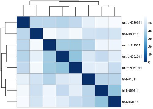
We can use many other plots to explore our data, using transformations such as principal components analysis (PCA) or multi-dimensional scaling (MDS) to look at the relationship between samples in a low dimensional space. Let’s create an MDS plot using our distance matrix:
library("ggplot2")

mds <- data.frame(cmdscale(sampleDistMatrix))
mds <- cbind(mds, as.data.frame(colData(rld)))
qplot(X1,X2,color=dex,shape=cell,data=mds)
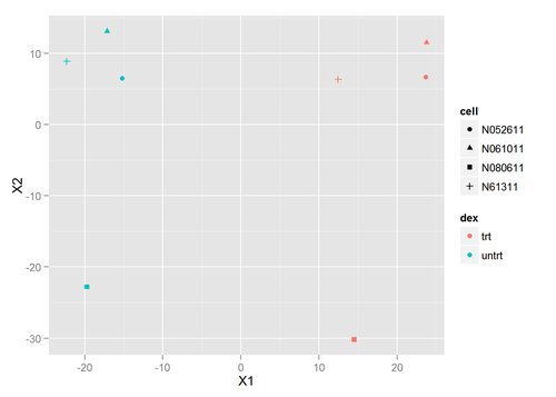
There’s clearly a difference between the treated and untreated samples - they separate nicely on the MDS plot. The separation of cell lines within each dex class also similar. Let’s go ahead and perform the DESeq analysis to find the significantly differentially expressed genes giving rise to this separation.
# for convenience set untreated as the first level in the dex factor
dds$dex <- relevel(dds$dex, "untrt")
dds <- DESeq(dds)
## estimating size factors
## estimating dispersions
## gene-wise dispersion estimates
## mean-dispersion relationship
## final dispersion estimates
## fitting model and testing(res <- results(dds))## log2 fold change (MAP): dex trt vs untrt
## Wald test p-value: dex trt vs untrt
## DataFrame with 64102 rows and 6 columns
## baseMean log2FoldChange lfcSE stat
## <numeric> <numeric> <numeric> <numeric>
## ENSG00000000003 708.60217 -0.37424998 0.09873107 -3.7906000
## ENSG00000000005 0.00000 NA NA NA
## ENSG00000000419 520.29790 0.20215551 0.10929899 1.8495642
## ENSG00000000457 237.16304 0.03624826 0.13684258 0.2648902
## ENSG00000000460 57.93263 -0.08523371 0.24654402 -0.3457140
## ... ... ... ... ...
## LRG_94 0 NA NA NA
## LRG_96 0 NA NA NA
## LRG_97 0 NA NA NA
## LRG_98 0 NA NA NA
## LRG_99 0 NA NA NA
## pvalue padj
## <numeric> <numeric>
## ENSG00000000003 0.0001502838 0.001217611
## ENSG00000000005 NA NA
## ENSG00000000419 0.0643763851 0.188306353
## ENSG00000000457 0.7910940556 0.907203245
## ENSG00000000460 0.7295576905 0.874422374
## ... ... ...
## LRG_94 NA NA
## LRG_96 NA NA
## LRG_97 NA NA
## LRG_98 NA NA
## LRG_99 NA NAsummary(res)##
## out of 33469 with nonzero total read count
## adjusted p-value < 0.1
## LFC > 0 (up) : 2646, 7.9%
## LFC < 0 (down) : 2251, 6.7%
## outliers [1] : 0, 0%
## low counts [2] : 15928, 48%
## (mean count < 5.3)
## [1] see 'cooksCutoff' argument of ?results
## [2] see 'independentFiltering' argument of ?resultsBy default we receive results for the last variable in our experimental design - in this case dex treatment. We can make different comparisons by calling results with a contrast parameter, e.g. considering two of our cell lines:
results(dds, contrast=c("cell", "N061011", "N61311"))## log2 fold change (MAP): cell N061011 vs N61311
## Wald test p-value: cell N061011 vs N61311
## DataFrame with 64102 rows and 6 columns
## baseMean log2FoldChange lfcSE stat pvalue
## <numeric> <numeric> <numeric> <numeric> <numeric>
## ENSG00000000003 708.60217 0.29055775 0.1360076 2.13633388 0.03265221
## ENSG00000000005 0.00000 NA NA NA NA
## ENSG00000000419 520.29790 -0.05069642 0.1491735 -0.33984871 0.73397047
## ENSG00000000457 237.16304 0.01474463 0.1816382 0.08117584 0.93530211
## ENSG00000000460 57.93263 0.20247610 0.2807312 0.72124547 0.47075850
## ... ... ... ... ... ...
## LRG_94 0 NA NA NA NA
## LRG_96 0 NA NA NA NA
## LRG_97 0 NA NA NA NA
## LRG_98 0 NA NA NA NA
## LRG_99 0 NA NA NA NA
## padj
## <numeric>
## ENSG00000000003 0.1961655
## ENSG00000000005 NA
## ENSG00000000419 0.9220321
## ENSG00000000457 0.9862824
## ENSG00000000460 0.8068941
## ... ...
## LRG_94 NA
## LRG_96 NA
## LRG_97 NA
## LRG_98 NA
## LRG_99 NAAn MA plot is useful to look at the relationship between expression and variance. Less highly expressed genes must have higher fold change to be considered significant, since the variance of their read counts is high.:
plotMA(res, ylim=c(-5,5))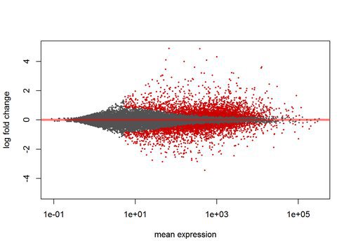
Annotating Results
So far our results from DESeq only identify genes by their Ensembl Gene ID. We can use annotation packages to see some more useful and friendly annotation.
library("AnnotationDbi")
library("org.Hs.eg.db")
## Loading required package: DBIConverting IDs with the native functions from the AnnotationDbi package is a bit cumbersome, so we provide the following convenience function (without explaining how exactly it works):
convertIDs <- function( ids, from, to, db, ifMultiple=c("putNA", "useFirst")) {
  stopifnot( inherits( db, "AnnotationDb" ) )
  ifMultiple <- match.arg( ifMultiple )
  suppressWarnings( selRes <- AnnotationDbi::select(
    db, keys=ids, keytype=from, columns=c(from,to) ) )
  if ( ifMultiple == "putNA" ) {
    duplicatedIds <- selRes[ duplicated( selRes[,1] ), 1 ]
    selRes <- selRes[ ! selRes[,1] %in% duplicatedIds, ]
  }
  return( selRes[ match( ids, selRes[,1] ), 2 ] )
}
We’ll add gene symbols and entrez IDs to our results and take a look at the top genes.
res$hgnc_symbol <- convertIDs(row.names(res), "ENSEMBL", "SYMBOL", org.Hs.eg.db)
res$entrezgene <- convertIDs(row.names(res), "ENSEMBL", "ENTREZID", org.Hs.eg.db)

resOrdered <- res[order(res$pvalue),]
head(resOrdered)
## log2 fold change (MAP): dex trt vs untrt
## Wald test p-value: dex trt vs untrt
## DataFrame with 6 rows and 8 columns
## baseMean log2FoldChange lfcSE stat
## <numeric> <numeric> <numeric> <numeric>
## ENSG00000152583 997.4398 4.316100 0.1724127 25.03354
## ENSG00000165995 495.0929 3.188698 0.1277441 24.96160
## ENSG00000101347 12703.3871 3.618232 0.1499441 24.13054
## ENSG00000120129 3409.0294 2.871326 0.1190334 24.12201
## ENSG00000189221 2341.7673 3.230629 0.1373644 23.51868
## ENSG00000211445 12285.6151 3.552999 0.1589971 22.34631
## pvalue padj hgnc_symbol entrezgene
## <numeric> <numeric> <character> <character>
## ENSG00000152583 2.637881e-138 4.627108e-134 SPARCL1 8404
## ENSG00000165995 1.597973e-137 1.401503e-133 CACNB2 783
## ENSG00000101347 1.195378e-128 6.441181e-125 SAMHD1 25939
## ENSG00000120129 1.468829e-128 6.441181e-125 DUSP1 1843
## ENSG00000189221 2.627083e-122 9.216332e-119 MAOA 4128
## ENSG00000211445 1.311440e-110 3.833996e-107 GPX3 2878Finally let’s save our results into a CSV format spreadsheet.
write.csv(as.data.frame(resOrdered), file="results.csv")Summary
This was a very quick run through some common steps in an RNA-Seq analysis and highlights relevant Bioconductor packages. Make sure to review the original tutorial for a more comprehensive explanation, and a look at filtering results, batch effects, and dealing with time series data:
Interacting with the BioHPC UCSC Genome Browser
(Adapted from the rtracklayer vignettes)
Other common workflows that Bioconductor is used for include ChIPSeq and association studies looking at mutations. In these types of work we often want to view data on a genome browser, plotting feature such as ChIP identified transcription factor binding sites against genomic sequence and other information.
BioHPC maintains a mirror of the UCSC Genome Browser at http://genome.biohpc.swmed.edu The Bioconductor rtracklayer pacakge allows us to interact directly with a UCSC browser, sending data from R to view as custom tracks within UCSC.
As a first example we’ll look for binding sites of NRSF on chromosome 1. There’s a known motif that we can find using the matchPatternfunction. The results will be put into a GenomicData object that can be used with rtracklayer,
library(BSgenome.Hsapiens.UCSC.hg19)## Loading required package: BSgenome
## Loading required package: rtracklayernrsfHits <- matchPattern("TCAGCACCATGGACAG", Hsapiens[["chr1"]])
length(nrsfHits)## [1] 2nrsfTrack <- GenomicData(ranges(nrsfHits), strand="+", chrom="chr1", genome = "hg19", asRangedData = FALSE)Generally, the quickest way to visualize the track is to start an rtracklayer browserSession and pass the track into the browseGenome function. However, this currently always calls the public UCSC server. We need to setup a session and manually create views and tracks in order to correctly target the BioHPC mirror.
library(rtracklayer)
session <- browserSession("UCSC", url="http://genome.biohpc.swmed.edu/cgi-bin/")
track(session, "NRSF" ) <- nrsfTrack
view <- browserView(session, range(nrsfTrack[1]) * -10)
Questions? Comments?
Please email biohpc-help@utsouthwestern.edu if you have any questions or comments regarding R or this training session.